Motivation
- Novel medical treatments are regularly discussed in social media
- Analyzing this data will help us understand:
- Concerns about the treatment
- Barriers to adoption
- Evolution of concerns over time
- This information will help us to:
- Learn how to communicate about novel treatments
- Understand how to address concerns
- Counsel patients about novel treatment options
Data
Source of Data:
- The data was collected by searching for relevant queries such as
male birth controlon Google, with the filtersite:reddit.com. - Around 74 posts over 12 years were identified, and the data was exported using PRAW.
- The data consists of the submissions with the comments in it. Also, the user history of the commenters was downloaded.
Data files
- submissions : 74 posts (in .pkl files)
- users: 21,627 user history of those who commented on the submissions (in .pkl files)
- Out of 41,792 comments read, 5179 comments had deleted user information.
- 22,099 unique users were found from all submissions.
Problem
We set out to answer the following questions, across four themes:
Timeline
- What years were users most engaged in the topic of male contraception?
- Are there users who engaged with the topic of male birth control over multiple years?
Geography
- Do users mention specific locations?
- What is the context around which users mention a location?
Sentiment
- What are the sentiments of the users when they write about male contraception?
- Has their sentiment shifted or remained the same over the years?
Topic Modeling
- What general topics can we identify in an unsupervised manner from the discussions on Reddit?
Methods
We attempted to answer these questions through the following methods:
Data Exploration and Visualization (Sanjana and Jae)
- Create histograms:
- Submissions by subreddit
- Submissions by year
- Comments by year
- Submissions by users
- Visualize geographic data:
- Number of mentions per US state
- Number of mentions per US state per 100,000 residents
Sentiment Analysis (Jae)
- Calculate the overall sentiment of each Reddit submission
- Depict words most occur in each negative and positive sentiment
- Visualize sentiment scores for all Reddit submissions to represent sentiment trend
Topic Model of Comments (Lei)
- Discover the abstract topics that frequently occur in Reddit comments
Results
Data Exploration
Number of Submissions by Subreddit
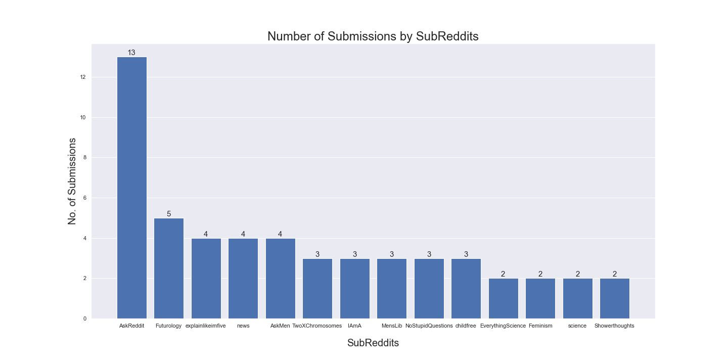
Reddit is a collection of subreddits, where each subreddit is a forum dedicated to a specific topic. From the data we collected, we observed that the highest number of submissions belonged to r/AskReddit, a popular subreddit for Redditors (users of Reddit) to ask and answer any kind of question. r/Futurology, a subreddit where people speculate about humanity, technology, and civilization, came in second.
Number of Submissions by Year
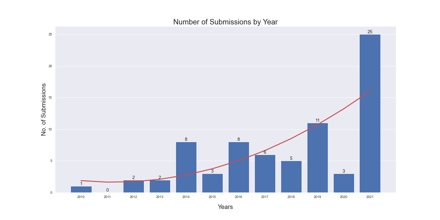
We observed that the number of submissions (posts on Reddit) increased over the years. This could be an artefact of collecting search results, or there could be more discourse about male contraception due to recent research advancements.
Number of comments by year
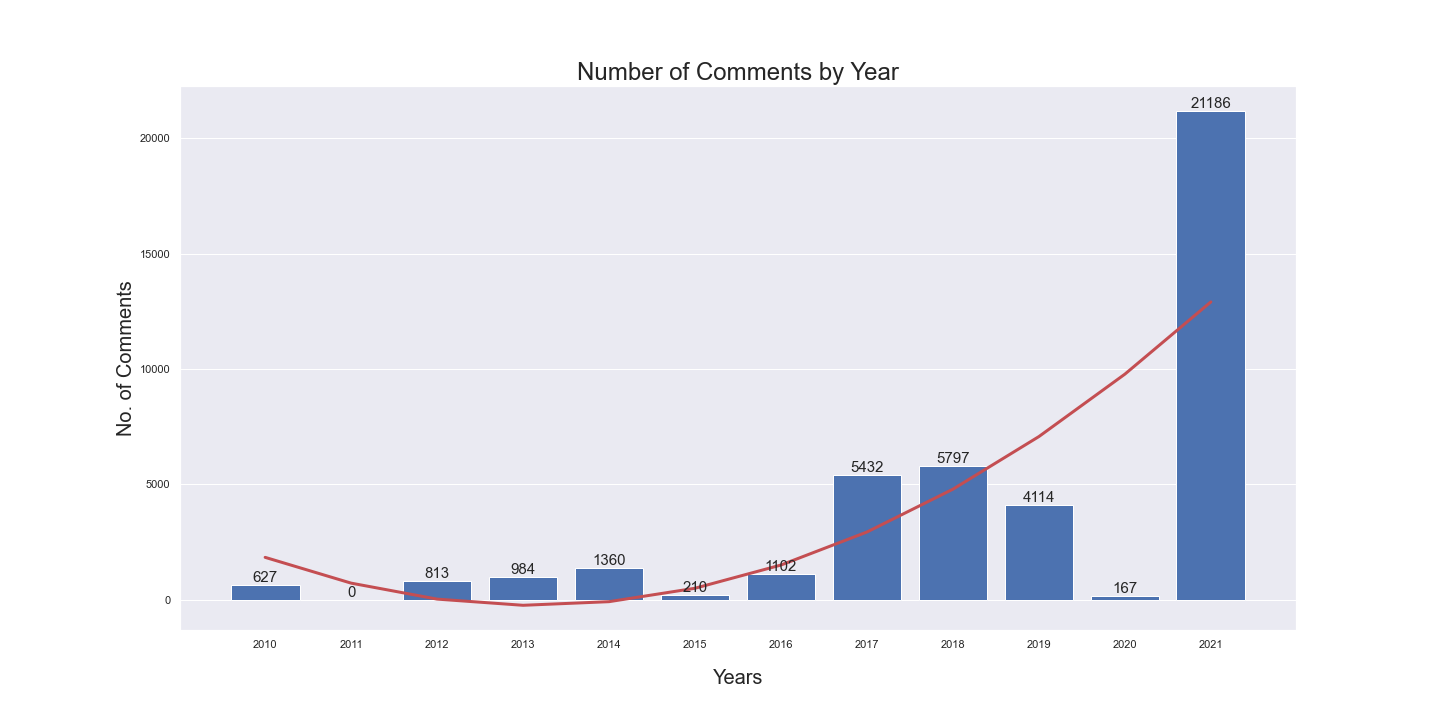
The number of comments under each submission also follows a similar trend. Interesting to note is the dip in 2020, right before the sharp rise in 2021.
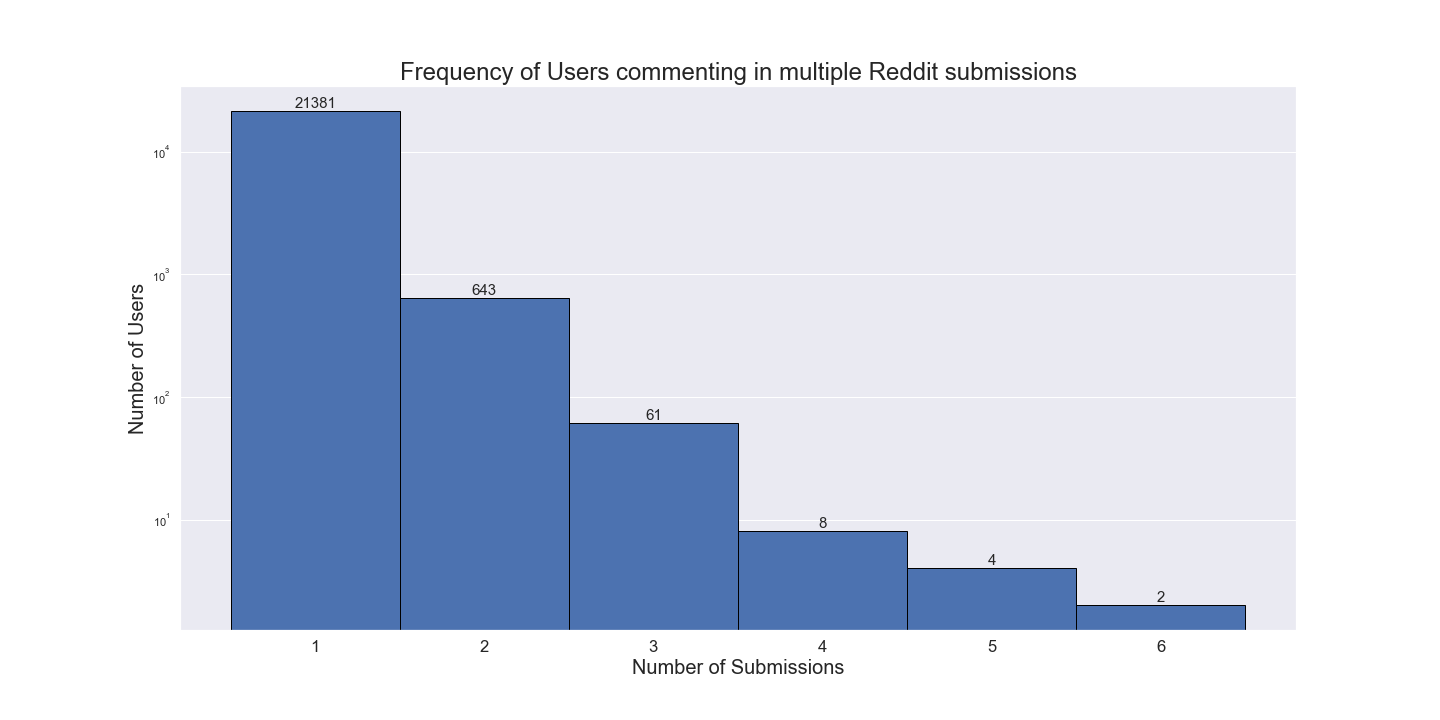
Users commenting in multiple posts
We drew histogram of users commenting in multiple Reddit submissions.
- From the 41,792 comments in 74 Reddit submissions, and excluding 5179 comments with deleted usernames, 22099 unique Reddit usernames were identified.
- 21381 Reddit usernames participated in only one Reddit submission.
- 643 Reddit usernames commented in two Reddit submissions.
- 61 Reddit usernames were found in three Reddit submissions, following with 8 Reddit usernames in four Reddit submissions, and 4 Reddit usernames in five Reddit submissions.
- 2 usernames commented in the six submissions, the maximum number of different Reddit submissions.
Click to expand for more details on histogram
Histogram of users commenting in multiple Reddit submissions.
Using matplotlib to represent the frequency of usernames present in multiple Reddit submissions.
- Created a list of usernames found in the comment section of each submission.
- Usernames with multiple comments were included only once, and deleted usernames were excluded.
- From the list of unique usernames for all Reddit submissions, the frequency of each username presents in all submissions were calculated.
- Using matplotlib, a histogram was plotted to represent the frequency of usernames commenting in multiple Reddit submissions.
Location Mentions
Number of Times US States Mentioned in Comments
We used SpaCy to perform Named Entity Recognition (NER) on the comments. USA was the most-mentioned country, and India was second. We decided to focus our work on US locations. We used the Nominatim API to get the US state names for the locations, thus filtering out non-US mentions. We also manually eliminated words such as “anesthesia” that were incorrectly tagged as locations during the NER phase.
California, Texas, New York, and Florida were the states with the most locations mentioned in comments.
But if we consider the number of mentions per 100k residents, we see a shift in the map. The District of Columbia tops the list, followed by North Dakota and Montana. Following is a graph of the mentions per 100k residents scaled by a factor of 100.
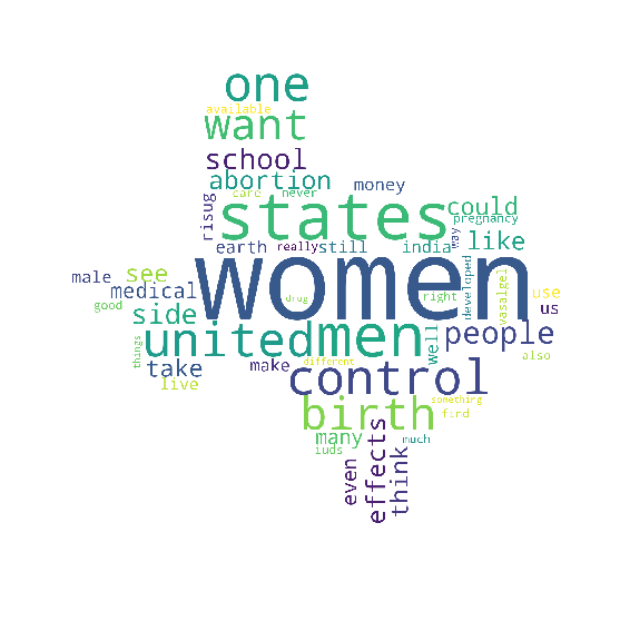
Top word used in the most-mentioned US states
The following pictures show the top words used in each state: California, Texas, New York, and Florida respectively.
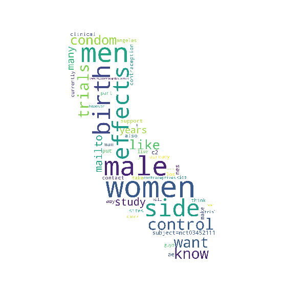
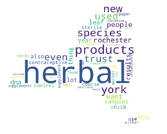
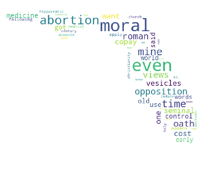
Some notable words:
- “NCT03452111”, an identifier for a clinical trial on gel-based male contraception, appears frequently which shows that people are paying attention to the research
- “Herbal” was a frequently used word with New York location mentions, perhaps in reference to herbal oral male contraceptives, but further analysis is necessary to be sure
- “Moral” is another interesting word appearance in Florida, and the comments will have to be analysed further to understand if there is any discussion around moral implications of contraceptives
Sentiment Analysis
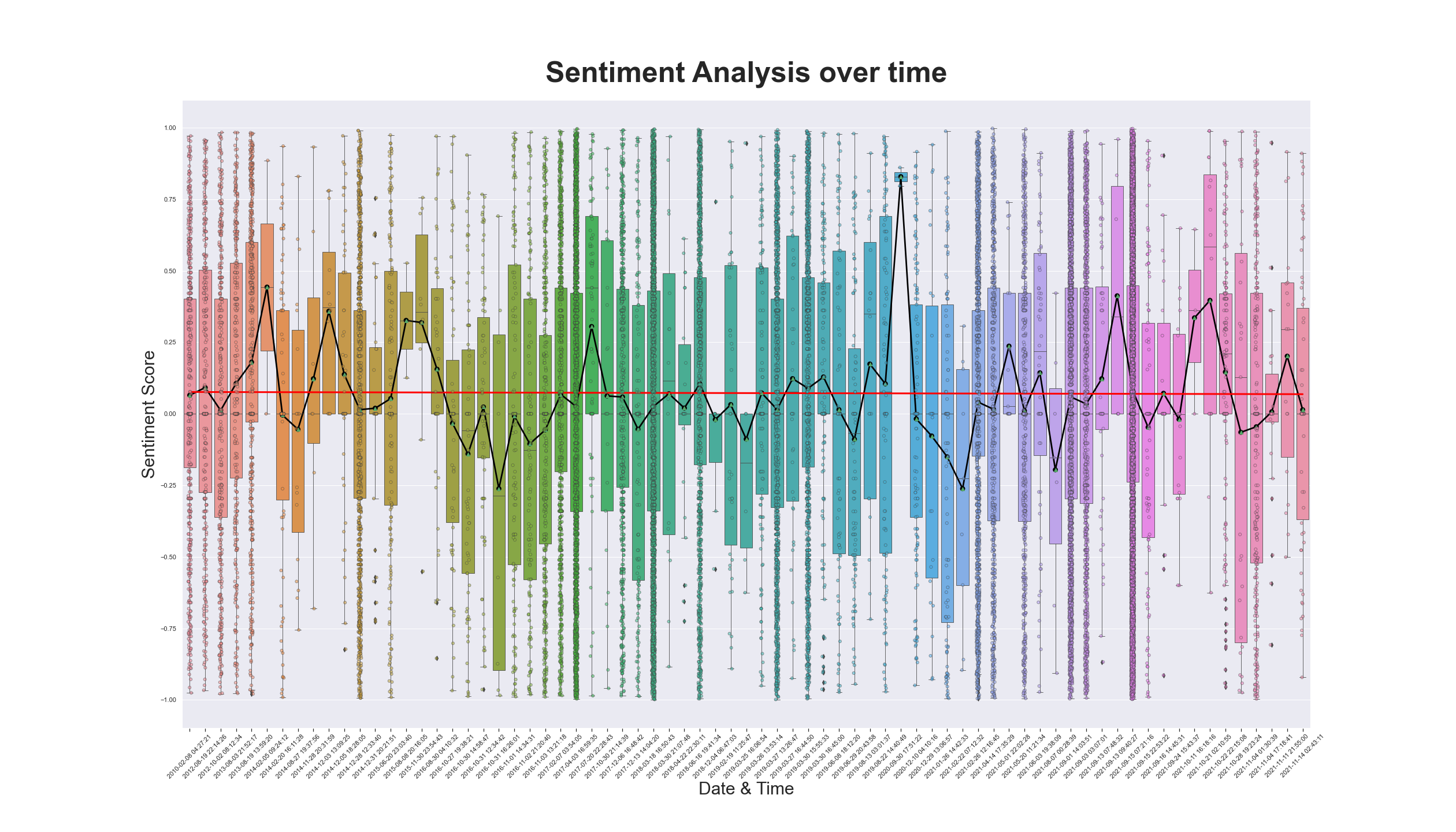
- From the 74 Reddit submissions, one submission was excluded for the lack of comments, and 73 submissions were included in the sentiment analysis.
- The first Reddit submission was dated February, 2010 and the last Reddit submission was dated November, 2021.
- From the data collected, the figure demonstrates a greater number of Reddit submission with an overall positive sentiment toward male contraception.
- In the trendline t1=0.0762 and t73 = 0.0686 with a delta of -0.0076 from the first Reddit submission and the last Reddit submission.
- Based on the data collected, it is inconclusive to determine if sentiment change for male contraception.
Click to expand for more details on sentiment analysis
Sentiment Analysis
Using VADER sentiment analysis, the overall sentiment of each Reddit submissions was calculated by analyzing all comments within the submission.
- Performed sentiment analysis of all comments in each Reddit submission by using (Valence Aware Dictionary and sEntiment Reasoner) VADER.
- A list was created to store the positive, negative, neutral and compound sentiment score for all comments of the Reddit submission.
- Comments with a compound sentiment scores greater than or equal to 0.05 was considered as positive sentiments, and compound sentiment scores less than or equal to -0.05 was considered as negative sentiments. Neutral sentiment ranged a compound sentiment scores between -0.05 and 0.05.
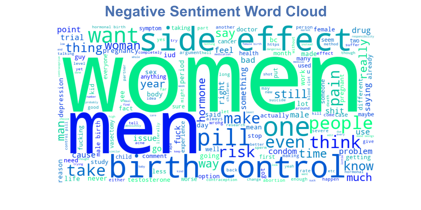
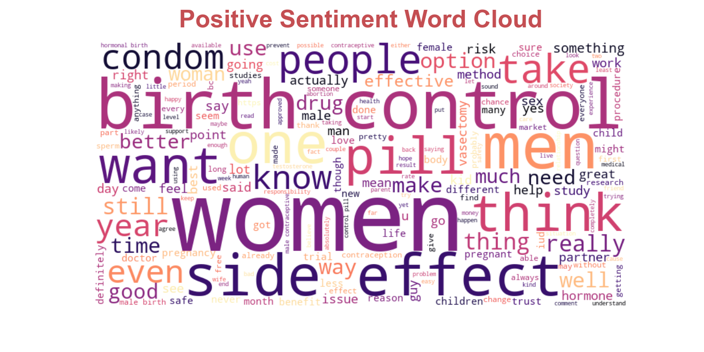
Word Cloud
Using WordCloud, comments with negative and positive sentiments were selected to create a word cloud to depicts words most found in each respective sentiment.
- Lists of comments with negative and positive sentiment were created, selecting comments with compound sentiment scores less than -0.9 and greater than 0.9 for their respective lists.
- All comments from both negative sentiments and positive sentiments were normalized by removing special characters, numbers and stopwords using (Natural Language Toolkit) NLTK.
- The resulting positive sentiment list of words and negative sentiment list of words were used to create their respective word cloud, using WordCloud.
Sentiment score Boxplot of all Reddit Submission
Using seaborn, boxplots of sentiment scores for all Reddit submissions was created using boxplot, stripplot, and pointplot, to represent all data points and a line graph of all means. A trendline using all means was also included in the figure.
- The lists of compound sentiment scores of all Reddit submissions were organized in chronological order.
- Seaborn was used to create a graphical representation of the result of the sentiment analysis, in chronological order in the x-axis and the sentiment score in the y-axis.
- Stripplot was used to plot all compound sentiment scores of all comments in each Reddit submission.
- Boxplot was used to create a box plot of each Reddit submission.
- Pointplot was used to create a line graph of the mean sentiment for each Reddit submission.
- A trendline of all mean scores was included using a numpy polyfit and poly1d.
Topic Model
Text Preprocessing
We will use the following techniques to create a corpus for our topic model and to make the model more interpretable:
- Tokenize documents and remove noise.
- Lemmatize the tokens.
- Compute bigrams.
- Compute a bag-of-words representation of the data.
Click to expand for more details on text preprocessing
Tokenize and Remove Noise
First, we tokenized the text (split the documents into tokens) using the tokenizer `gensim.utils.tokenize()` from Gensim. We removed the following tokens or comments as they don't tend to be useful, and the comments contain a lot of them.
- stopwords: gensim.parsing.preprocessing.STOPWORDS
- single character tokens and numeric tokens
- URLs: regular expression, `r'http\S+'`
- common and rare words: filter out words that occur less than 5 documents, or more than 30% of the documents.
- [deleted] comments
Lemmatize the Tokens
We found some words with the same meaning could occur in one topic, especially gender words. For example, our topic model could generate a topic containing "female", "women", and "woman" at the same time. Gender words are important for our model because we are studying topics like birth control, but words with the same meaning could appear in a topic, which will harm the informativeness of our topic model.
We use the WordNet lemmatizer from NLTK, "nltk.stem.wordnet.WordNetLemmatizer". A lemmatizer could produce more readable words and help our topic model generate more informative topics. This is very desirable in topic modeling.
Bigrams
We find bigrams in the documents(comments) with `gensim.models.Phrases`. Bigrams are sets of two adjacent words. Using bigrams we can get phrases like "birth_control" in our output (spaces are replaced with underscores); without bigrams we would only get "birth" and "control".
Then, add bigrams into our corpus, because we would like to keep the words "birth" and "control" as well as the bigram "birth_control". The following block shows part of phrases found by the bigram model
['fda_approval', 'lasts_years', 'test_subjects', 'sperm_count', 'birth_control', 'family_planning', 'tl_dr', 'reproductive_organs', 'shoot_blanks', 'bullet_proof', 'proof_vest', 'sex_drive', 'paying_child', 'child_support', 'hell_yes', 'female_birth', 'protect_stds', 'male_birth', 'proven_safe', 'birth_controls', 'shooting_blanks', 'approved_fda', 'want_kids', 'hormonal_birth', 'use_condoms', 'shoot_bulletproof', ...]
The output of topic model will show that bigrams indeed improved our model to generate better topics. For instance, some topics contains bigrams `birth_control` and `male_birth`.
Bag-of-words
Bag-of-words model is an approach to represent a document as a vector. Under the bag-of-words model each document is represented by a vector containing the frequency counts of each word in the dictionary.
For example, assume we have a dictionary containing the words `['coffee', 'milk', 'sugar', 'spoon']`. A document consisting of the string "coffee milk coffee" would then be represented by the vector `[2, 1, 0, 0]`. One of the main properties of the bag-of-words model is that it completely ignores the order of the tokens in the document that is encoded, which is where the name bag-of-words comes from.
Here, we created a dictionary representation of the documents with `gensim.corpora.Dictionary` and `doc2bow()` method could create a corpus as the input of our topic model.
Topic Model Training
Our topic model is based on Latent Dirichlet allocation (LDA). Hyperparameter tuning shows the when the number of topics is 8, the LDA model performs best.
Click to see the details on training and hyperparameter tuning
LDA is a generative statistical model that allows sets of observations to be explained by unobserved groups that explain why some parts of the data are similar. We can build a LDA topic model using `gensim.models.Lda`. We will first discuss how to set some of the training parameters.
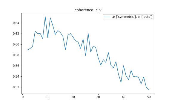
First of all, the elephant in the room: how many topics do we need? Let’s perform a series of sensitivity tests to help determine the following model hyperparameters
- Number of Topics (K)
- Dirichlet hyperparameter (alpha): Document-Topic Density
- Dirichlet hyperparameter (beta): Word-Topic Density
We’ll perform these tests in sequence, one parameter at a time by keeping others constant and run them over the two different validation corpus sets. We'll use topic coherence, 'C_v', as our choice of metric for performance comparison. We found the default setting, "alpha='symmetric', beta='auto'", perform best, so we will keep this setting to explore the optimal number of topics.
Pick the model that gave the highest 'C_v'. In this case, we picked K=8 with highest average topic coherence 0.6425.
Output of Topic Model
Let’s take a look at these 8 topics generated by our topic models. Each topic is a combination of keywords, and each keyword contributes a certain weightage to the topic. The following cell shows the 8 topics.
Topic 1: 0.057*"female" + 0.034*"pill" + 0.029*"male" + 0.023*"effect" + 0.021*"birth_control" + 0.011*"think" + 0.009*"want" + 0.009*"taking" + 0.008*"control" + 0.007*"like"

Topic 2: 0.039*"male" + 0.038*"female" + 0.021*"effect" + 0.014*"birth_control" + 0.010*"condom" + 0.009*"risk" + 0.009*"control" + 0.008*"option" + 0.008*"people" + 0.007*"use"

Topic 3: 0.028*"male" + 0.025*"yes" + 0.021*"child" + 0.020*"condom" + 0.020*"want" + 0.016*"female" + 0.009*"think" + 0.009*"kid" + 0.008*"people" + 0.008*"option"

Topic 4: 0.018*"effect" + 0.015*"male" + 0.014*"testosterone" + 0.012*"hormone" + 0.010*"pill" + 0.009*"people" + 0.009*"drug" + 0.009*"female" + 0.008*"like" + 0.008*"level"

Topic 5: 0.019*"like" + 0.018*"iud" + 0.017*"year" + 0.012*"time" + 0.011*"pain" + 0.011*"pill" + 0.010*"day" + 0.010*"period" + 0.009*"got" + 0.008*"month"

Topic 6: 0.015*"like" + 0.010*"comment" + 0.010*"thing" + 0.010*"male" + 0.010*"know" + 0.009*"people" + 0.008*"right" + 0.007*"question" + 0.007*"sure" + 0.007*"fucking"

Topic 7: 0.023*"control" + 0.018*"sperm" + 0.017*"study" + 0.015*"removed" + 0.014*"male" + 0.013*"pill" + 0.013*"like" + 0.013*"effect" + 0.012*"trial" + 0.012*"male_birth"

Topic 8: 0.048*"vasectomy" + 0.014*"procedure" + 0.012*"reversible" + 0.009*"vasalgel" + 0.008*"year" + 0.008*"think" + 0.007*"absolutely" + 0.007*"yeah" + 0.007*"surgery" + 0.007*"kid"
Topic Visualization
The above results are hard to read, so we created an interactive graph to interpret the topics, which provides:
- a left panel that depicts a global view of the model (how prevalent each topic is and how topics relate to each other);
- a right panel containing a bar chart – the bars represent the terms that are most useful in interpreting the topic currently selected (what the meaning of each topic is).
For instance, if we choose topic 1 on the left panel, we can see the top most relevant terms for Topic 1 contains, female, pill, male, effect, birth_control, etc. And if we choose the term “pill”, the right panel will show the conditional topic distribution given the term “pill”. Obviously, “pill” is mentioned more in topic 1 than other topics.
Click to expand for more details on topics' visualization
We created this interactive graph with `pyLDAvis` package to interpret the topics.
On the left, the topics are plotted as circles, whose centers are defined by the computed distance between topics (projected into 2 dimensions). The prevalence of each topic is indicated by the circle’s area. On the right, two juxtaposed bars showing the topic-specific frequency of each term (in red) and the corpus-wide frequency (in blueish gray). When no topic is selected, the right panel displays the top 30 most salient terms for the dataset.
Relevance is denoted by λ, the weight assigned to the probability of a term in a topic relative to its lift. When λ = 1, the terms are ranked by their probabilities within the topic (the ‘regular’ method) while when λ = 0, the terms are ranked only by their lift. The interface allows to adjust the value of λ between 0 and 1.
For more details about topics' visualization, please see this paper, LDAvis: A method for visualizing and interpreting topics.
Topic Interpretation
Then, let’s interpret the output of our topic model. We tried to give an interpretation for each topic, which is shown below. Not all generated topics are interpretable, for instance, it’s hard to interpret the combination of the 10 words in topic 6.
- Effect of birth control pill
- Risk of birth control methods
- People want kids
- Effect of testosterone for male
- IUD pain long term
- Study of male birth control
- Vasectomy reversal surgery, and vasalgel (a new male reversible contraceptive).
Conclusion
-
The histograms in data exploration shows that male contraceptives has been a topic of interest in the recent years compared to the early 2010’s with the greatest number of posts and comments in 2021. Still, only a small number of users participate in multiple number of submissions with the greater majority of users were only in one male contraceptive Reddit post.
-
The majority of the comments were identified to originate from the United States, especially states with major metropolitan cities like California, Texas, Florida, and New York.
-
The sentiment analysis demonstrates a slight positive to neutral sentiment towards male contraceptives. Furthermore, the sentiment score has remained stable throughout the 12 years time frame, which is likely due to the absence of a male contraceptive product.
-
The generated topics regarding contraceptives are related to possible side effects, and family planning, and new male contraceptive product.